
Basic Usage Examples#
This notebook walks through representative data processing patterns to show what you can do with limulus.
import limulus
import pandas as pd
import polars as pl

iris_data = pd.read_csv('https://raw.githubusercontent.com/mwaskom/seaborn-data/master/iris.csv')

session = limulus.Session()
session.loads({"iris": iris_data})
Example 1: Common Syntax#
session.submit("""
data ratios;
  set iris;
  sepal_ratio = round(sepal_length / sepal_width, 0.01);
  petal_area = round(petal_length * petal_width, 0.01);
  keep species sepal_length sepal_width sepal_ratio petal_area;
run;
""")

print(pl.from_arrow(session["ratios"]).head(5))
shape: (5, 5)
┌──────────────┬─────────────┬─────────┬─────────────┬────────────┐
│ sepal_length ┆ sepal_width ┆ species ┆ sepal_ratio ┆ petal_area │
│ ---          ┆ ---         ┆ ---     ┆ ---         ┆ ---        │
│ f64          ┆ f64         ┆ str     ┆ f64         ┆ f64        │
╞══════════════╪═════════════╪═════════╪═════════════╪════════════╡
│ 5.1          ┆ 3.5         ┆ setosa  ┆ 1.46        ┆ 0.28       │
│ 4.9          ┆ 3.0         ┆ setosa  ┆ 1.63        ┆ 0.28       │
│ 4.7          ┆ 3.2         ┆ setosa  ┆ 1.47        ┆ 0.26       │
│ 4.6          ┆ 3.1         ┆ setosa  ┆ 1.48        ┆ 0.3        │
│ 5.0          ┆ 3.6         ┆ setosa  ┆ 1.39        ┆ 0.28       │
└──────────────┴─────────────┴─────────┴─────────────┴────────────┘
Example 2: DO–END and Multiple Output Datasets#
session.submit("""
data large_petal small_petal;
  set iris;
  if petal_length > 2.0 then do ;
    size_group = "large" ;
    output large_petal;
  end ;
  else do ;
    size_group = "small" ;
    output small_petal;
  end ;
run;
""")

# 2 ways convert to polars
print(pl.from_arrow(session["large_petal"]).head(3))
print(session.dataset("small_petal").to_polars().head(3))
shape: (3, 6)
┌──────────────┬─────────────┬──────────────┬─────────────┬────────────┬────────────┐
│ sepal_length ┆ sepal_width ┆ petal_length ┆ petal_width ┆ species    ┆ size_group │
│ ---          ┆ ---         ┆ ---          ┆ ---         ┆ ---        ┆ ---        │
│ f64          ┆ f64         ┆ f64          ┆ f64         ┆ str        ┆ str        │
╞══════════════╪═════════════╪══════════════╪═════════════╪════════════╪════════════╡
│ 7.0          ┆ 3.2         ┆ 4.7          ┆ 1.4         ┆ versicolor ┆ large      │
│ 6.4          ┆ 3.2         ┆ 4.5          ┆ 1.5         ┆ versicolor ┆ large      │
│ 6.9          ┆ 3.1         ┆ 4.9          ┆ 1.5         ┆ versicolor ┆ large      │
└──────────────┴─────────────┴──────────────┴─────────────┴────────────┴────────────┘
shape: (3, 6)
┌──────────────┬─────────────┬──────────────┬─────────────┬─────────┬────────────┐
│ sepal_length ┆ sepal_width ┆ petal_length ┆ petal_width ┆ species ┆ size_group │
│ ---          ┆ ---         ┆ ---          ┆ ---         ┆ ---     ┆ ---        │
│ f64          ┆ f64         ┆ f64          ┆ f64         ┆ str     ┆ str        │
╞══════════════╪═════════════╪══════════════╪═════════════╪═════════╪════════════╡
│ 5.1          ┆ 3.5         ┆ 1.4          ┆ 0.2         ┆ setosa  ┆ small      │
│ 4.9          ┆ 3.0         ┆ 1.4          ┆ 0.2         ┆ setosa  ┆ small      │
│ 4.7          ┆ 3.2         ┆ 1.3          ┆ 0.2         ┆ setosa  ┆ small      │
└──────────────┴─────────────┴──────────────┴─────────────┴─────────┴────────────┘
Example 3: BY Group Processing (RETAIN + FIRST. / LAST.)#
session.submit("""
data avg_petal;
  set ratios;
  by species;
  retain area_sum 0 area_count 0;

  if first.species then do;
    area_sum = 0;
    area_count = 0;
  end;

  area_sum + petal_area;
  area_count + 1;

  if last.species then do;
    avg_petal_area = round(area_sum / area_count, 0.01);
    output;
  end;

  keep species area_count avg_petal_area;
run;
""")

print(session.dataset("avg_petal").to_polars())
shape: (3, 3)
┌────────────┬────────────┬────────────────┐
│ species    ┆ area_count ┆ avg_petal_area │
│ ---        ┆ ---        ┆ ---            │
│ str        ┆ f64        ┆ f64            │
╞════════════╪════════════╪════════════════╡
│ setosa     ┆ 50.0       ┆ 0.37           │
│ versicolor ┆ 50.0       ┆ 5.72           │
│ virginica  ┆ 50.0       ┆ 11.3           │
└────────────┴────────────┴────────────────┘
Example 4: Joining Data#
# Create a species lookup table
species_info = pl.DataFrame({
    "species": ["setosa", "versicolor", "virginica"],
    "category": ["small", "medium", "large"],
})
session.loads({"species_info": species_info})

session.submit("""
/* Vertical concatenation */
data iris_doubled ;
  set iris(in=in1) iris ;
  if in1 = 1 then tag = "first" ;
  else tag = "second" ;
run ;

/* Horizontal join */
data iris_labeled;
  merge iris(in=in1) species_info;
  by species ;
  if in1 ;
run;
""")

print("rows:", session["iris_doubled"].shape[0])
print(session.dataset("iris_labeled").to_polars().head(5))
rows: 300
shape: (5, 6)
┌──────────────┬─────────────┬──────────────┬─────────────┬─────────┬──────────┐
│ sepal_length ┆ sepal_width ┆ petal_length ┆ petal_width ┆ species ┆ category │
│ ---          ┆ ---         ┆ ---          ┆ ---         ┆ ---     ┆ ---      │
│ f64          ┆ f64         ┆ f64          ┆ f64         ┆ str     ┆ str      │
╞══════════════╪═════════════╪══════════════╪═════════════╪═════════╪══════════╡
│ 5.1          ┆ 3.5         ┆ 1.4          ┆ 0.2         ┆ setosa  ┆ small    │
│ 4.9          ┆ 3.0         ┆ 1.4          ┆ 0.2         ┆ setosa  ┆ small    │
│ 4.7          ┆ 3.2         ┆ 1.3          ┆ 0.2         ┆ setosa  ┆ small    │
│ 4.6          ┆ 3.1         ┆ 1.5          ┆ 0.2         ┆ setosa  ┆ small    │
│ 5.0          ┆ 3.6         ┆ 1.4          ┆ 0.2         ┆ setosa  ┆ small    │
└──────────────┴─────────────┴──────────────┴─────────────┴─────────┴──────────┘
Example 5: Integration with Python#
Here we combine Python processing before and after the Data Step.
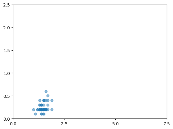
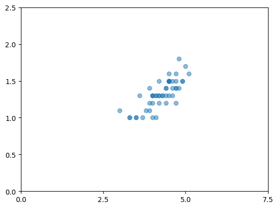
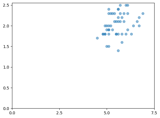
As an example, we run a loop to compute sepal area by species and display scatter plots with matplotlib.
import matplotlib.pyplot as plt

for sp in ["setosa", "versicolor", "virginica"]:
    session.submit(f"""
    data sepal_{sp} ;
      set iris ;
      where species = "{sp}" ;
      sepal_area = round(sepal_length * sepal_width, 0.01) ;
      keep species sepal_area petal_length petal_width;
    run ;
    """)

    out = session[f"sepal_{sp}"].to_pandas()
    print(f"species={sp}: {len(out)} rows, mean sepal_area={out['sepal_area'].mean():.2f}")

    plt.figure()
    plt.scatter(out["petal_length"], out["petal_width"], alpha=0.5)
    plt.yticks([0, 0.5, 1.0, 1.5, 2.0, 2.5])
    plt.xticks([0, 2.5, 5.0, 7.5])
    plt.show()
    plt.close()
species=setosa: 50 rows, mean sepal_area=17.26
species=versicolor: 50 rows, mean sepal_area=16.53
species=virginica: 50 rows, mean sepal_area=19.68
apply() calls a Python function by name inside a data step expression. It supports builtins, dotted module functions, and local helper functions that are available when execution starts.
If you need a function that is not available in the built-in function set, you can use apply() to handle it.
However, apply() uses Python-side row-wise processing and can reduce performance, so use it with care on large datasets.
def my_func1(x,y):
	return x + y

def my_func2(x, y):
	return x[:y]


session.submit("""
data apply_sample;
  set iris;
  sum_length = apply("my_func1", sepal_length, petal_length);
  sub_txt = apply("my_func2", species, 3);
  rand_val = apply("numpy.random.normal", 0, 1);
  keep species sum_length sub_txt rand_val;
run ;
""")

print(session.dataset("apply_sample").to_polars().head(5))
shape: (5, 4)
┌─────────┬────────────┬─────────┬───────────┐
│ species ┆ sum_length ┆ sub_txt ┆ rand_val  │
│ ---     ┆ ---        ┆ ---     ┆ ---       │
│ str     ┆ f64        ┆ str     ┆ f64       │
╞═════════╪════════════╪═════════╪═══════════╡
│ setosa  ┆ 6.5        ┆ set     ┆ 0.275952  │
│ setosa  ┆ 6.3        ┆ set     ┆ 0.030283  │
│ setosa  ┆ 6.0        ┆ set     ┆ -1.390121 │
│ setosa  ┆ 6.1        ┆ set     ┆ -1.653369 │
│ setosa  ┆ 6.4        ┆ set     ┆ -0.439669 │
└─────────┴────────────┴─────────┴───────────┘
Example 6: Metadata#
You can assign label information as Arrow metadata.
However, if additional processing is performed afterward, the metadata may currently be dropped unintentionally.For this reason, labels should be applied immediately before producing the final output.
session.submit("""
data iris_labels(label="Iris sample");
  set iris(obs=3);
  label sepal_length = "Sepal Length";
run;
""")

print(session.dataset("iris_labels").to_arrow().schema)
sepal_length: double
  -- field metadata --
  label: 'Sepal Length'
sepal_width: double
petal_length: double
petal_width: double
species: string
-- schema metadata --
memlabel: 'Iris sample'
Table metadata can be retrieved from dictionary.tables or dictionary.columns.
session.submit("""
data tables;
  set dictionary.tables;
  where memname = "IRIS_LABELS";
run ;

data columns;
  set dictionary.columns;
  where memname = "IRIS_LABELS";
run ;
"""
)

print(session.dataset("tables").to_polars())
print(session.dataset("columns").to_polars())
shape: (1, 6)
┌─────────┬─────────────┬─────────┬─────────────┬──────┬──────┐
│ LIBNAME ┆ MEMNAME     ┆ MEMTYPE ┆ MEMLABEL    ┆ NOBS ┆ NVAR │
│ ---     ┆ ---         ┆ ---     ┆ ---         ┆ ---  ┆ ---  │
│ str     ┆ str         ┆ str     ┆ str         ┆ i64  ┆ i64  │
╞═════════╪═════════════╪═════════╪═════════════╪══════╪══════╡
│ WORK    ┆ IRIS_LABELS ┆ DATA    ┆ Iris sample ┆ 3    ┆ 5    │
└─────────┴─────────────┴─────────┴─────────────┴──────┴──────┘
shape: (5, 9)
┌─────────┬─────────────┬─────────┬──────────────┬───┬────────┬──────────────┬────────┬──────────┐
│ LIBNAME ┆ MEMNAME     ┆ MEMTYPE ┆ NAME         ┆ … ┆ VARNUM ┆ LABEL        ┆ FORMAT ┆ INFORMAT │
│ ---     ┆ ---         ┆ ---     ┆ ---          ┆   ┆ ---    ┆ ---          ┆ ---    ┆ ---      │
│ str     ┆ str         ┆ str     ┆ str          ┆   ┆ i64    ┆ str          ┆ str    ┆ str      │
╞═════════╪═════════════╪═════════╪══════════════╪═══╪════════╪══════════════╪════════╪══════════╡
│ WORK    ┆ IRIS_LABELS ┆ DATA    ┆ sepal_length ┆ … ┆ 1      ┆ Sepal Length ┆        ┆          │
│ WORK    ┆ IRIS_LABELS ┆ DATA    ┆ sepal_width  ┆ … ┆ 2      ┆              ┆        ┆          │
│ WORK    ┆ IRIS_LABELS ┆ DATA    ┆ petal_length ┆ … ┆ 3      ┆              ┆        ┆          │
│ WORK    ┆ IRIS_LABELS ┆ DATA    ┆ petal_width  ┆ … ┆ 4      ┆              ┆        ┆          │
│ WORK    ┆ IRIS_LABELS ┆ DATA    ┆ species      ┆ … ┆ 5      ┆              ┆        ┆          │
└─────────┴─────────────┴─────────┴──────────────┴───┴────────┴──────────────┴────────┴──────────┘
Example 7: put, input, and type conversion#
For put and input, the following commonly used forms are currently supported.
best., w.d., zw.d., commaw.d., e8601da., e8601dt., yymmdd6., yymmdd8., yymmdd10., time.
Simple dictionary-based conversion is supported as a custom format.
When input is used with date/time formats, the result is a datetime-type value rather than a numeric value.
For type conversions other than put and input, you can use the dataset method astype (or cast).
If you need to keep the original column, specify alias= to leave the original column unchanged and add a new column with the given name.
session.register_format("myfmt", {10: "ten"})

session.submit("""
data put_input;
  set iris;
  slength_str = put(sepal_length, best.);
  num = input("10", best.);
  num_str = put(num, myfmt.);
  date = input("2024-01-01", e8601da.);
  date_str = put(date, e8601da.);
  keep sepal_length slength_str num num_str date date_str;
run;
"""
)

session.dataset("put_input").astype({"slength_str": "float64"}, alias="slength_num")

print(pl.from_arrow(session["put_input"]).head(5))
shape: (5, 7)
┌──────────────┬─────────────┬──────┬─────────┬────────────┬────────────┬─────────────┐
│ sepal_length ┆ slength_str ┆ num  ┆ num_str ┆ date       ┆ date_str   ┆ slength_num │
│ ---          ┆ ---         ┆ ---  ┆ ---     ┆ ---        ┆ ---        ┆ ---         │
│ f64          ┆ str         ┆ f64  ┆ str     ┆ date       ┆ str        ┆ f64         │
╞══════════════╪═════════════╪══════╪═════════╪════════════╪════════════╪═════════════╡
│ 5.1          ┆ 5.1         ┆ 10.0 ┆ ten     ┆ 2024-01-01 ┆ 2024-01-01 ┆ 5.1         │
│ 4.9          ┆ 4.9         ┆ 10.0 ┆ ten     ┆ 2024-01-01 ┆ 2024-01-01 ┆ 4.9         │
│ 4.7          ┆ 4.7         ┆ 10.0 ┆ ten     ┆ 2024-01-01 ┆ 2024-01-01 ┆ 4.7         │
│ 4.6          ┆ 4.6         ┆ 10.0 ┆ ten     ┆ 2024-01-01 ┆ 2024-01-01 ┆ 4.6         │
│ 5.0          ┆ 5           ┆ 10.0 ┆ ten     ┆ 2024-01-01 ┆ 2024-01-01 ┆ 5.0         │
└──────────────┴─────────────┴──────┴─────────┴────────────┴────────────┴─────────────┘
Example 8: Column-Oriented API and Session Helpers#
It is intended to make it easier to express proc sytep operations and column-oriented processing needed for high-performance workloads.
This part is still under active development, and additional functionality will be added in upcoming updates. Column-oriented helpers on Session and DatasetView currently require exact column names and are case-sensitive.
After obtaining a dataset view with session.dataset(), you can use methods such as sort(), select() (for column selection and reordering), and astype() for type conversion.
(
session.dataset("iris")
    .sort(by="species", out="iris_s")
    .select(["species","sepal_length"])
    .astype({"sepal_length": "float32"})
)

print(session.dataset("iris_s").to_polars().head(3))
shape: (3, 2)
┌─────────┬──────────────┐
│ species ┆ sepal_length │
│ ---     ┆ ---          │
│ str     ┆ f32          │
╞═════════╪══════════════╡
│ setosa  ┆ 5.1          │
│ setosa  ┆ 4.9          │
│ setosa  ┆ 4.7          │
└─────────┴──────────────┘
Row-oriented processing is generally less efficient than column-oriented processing. To handle large datasets, we provide a column-oriented API (please note that while the API structure is currently available, performance optimizations are planned for future updates). The assign method is designed for simple variable manipulation. It supports assignments using constants or functions, as well as conditional logic using “case when” statements.
session.dataset("iris").assign(out="iris_a",
                               lit1 = 1,
                               lit2 = "'str'",
                               num1 = "sepal_length * 2",
                               str1 = "substr(species, 1, 3)",
                               group = "case when sepal_length > 5.0 then 'long' else 'short' end"
                               ).select(["species", "sepal_length","lit1", "lit2", "num1", "str1", "group"])

print(session.dataset("iris_a").to_polars().head())
shape: (5, 7)
┌─────────┬──────────────┬──────┬──────┬──────┬──────┬───────┐
│ species ┆ sepal_length ┆ lit1 ┆ lit2 ┆ num1 ┆ str1 ┆ group │
│ ---     ┆ ---          ┆ ---  ┆ ---  ┆ ---  ┆ ---  ┆ ---   │
│ str     ┆ f64          ┆ i32  ┆ str  ┆ f64  ┆ str  ┆ str   │
╞═════════╪══════════════╪══════╪══════╪══════╪══════╪═══════╡
│ setosa  ┆ 5.1          ┆ 1    ┆ str  ┆ 10.2 ┆ set  ┆ long  │
│ setosa  ┆ 4.9          ┆ 1    ┆ str  ┆ 9.8  ┆ set  ┆ short │
│ setosa  ┆ 4.7          ┆ 1    ┆ str  ┆ 9.4  ┆ set  ┆ short │
│ setosa  ┆ 4.6          ┆ 1    ┆ str  ┆ 9.2  ┆ set  ┆ short │
│ setosa  ┆ 5.0          ┆ 1    ┆ str  ┆ 10.0 ┆ set  ┆ short │
└─────────┴──────────────┴──────┴──────┴──────┴──────┴───────┘
We provide basic functionality for transposing data; however, this is primarily intended as a supportive support feature. For more complex operations or scenarios requiring higher efficiency, we recommend considering processing with Arrow or Polars.
import pyarrow as pa
test = pa.table({
                "grp": ["a", "a", "b"],
                "visit": ["v1", "v2", "v1"],
                "score": [10, 20, 30],
            })
session.loads({"test": test})

session.dataset("test").transpose(out="test_t", by=["grp"], id="visit", var=["score"])

print(session.dataset("test_t").to_polars())
shape: (2, 3)
┌─────┬─────┬──────┐
│ grp ┆ v1  ┆ v2   │
│ --- ┆ --- ┆ ---  │
│ str ┆ i64 ┆ i64  │
╞═════╪═════╪══════╡
│ a   ┆ 10  ┆ 20   │
│ b   ┆ 30  ┆ null │
└─────┴─────┴──────┘
Data creation using SQL queries is supported through session.sql.
The SQL syntax follows the Polars SQL implementation.
session.sql(
    """
    create table iris_summary as
    select
        species,
        round(avg(sepal_length), 2) as avg_sepal_length,
        round(avg(petal_length), 2) as avg_petal_length
    from iris
    group by species
    """
)
print(session.dataset("iris_summary").to_polars())
shape: (3, 3)
┌────────────┬──────────────────┬──────────────────┐
│ species    ┆ avg_sepal_length ┆ avg_petal_length │
│ ---        ┆ ---              ┆ ---              │
│ str        ┆ f64              ┆ f64              │
╞════════════╪══════════════════╪══════════════════╡
│ versicolor ┆ 5.94             ┆ 4.26             │
│ virginica  ┆ 6.59             ┆ 5.55             │
│ setosa     ┆ 5.01             ┆ 1.46             │
└────────────┴──────────────────┴──────────────────┘
If you have code saved in a text file, you can load and execute it using session.include.
from pathlib import Path
from tempfile import TemporaryDirectory

with TemporaryDirectory() as tmpdir:
    script = Path(tmpdir) / "include.txt"
    script.write_text("""
data inc_sample;
  set iris(obs=3);
run;
""", encoding="utf-8")

    session.include(script)

print(session.dataset("inc_sample").to_polars())
shape: (3, 5)
┌──────────────┬─────────────┬──────────────┬─────────────┬─────────┐
│ sepal_length ┆ sepal_width ┆ petal_length ┆ petal_width ┆ species │
│ ---          ┆ ---         ┆ ---          ┆ ---         ┆ ---     │
│ f64          ┆ f64         ┆ f64          ┆ f64         ┆ str     │
╞══════════════╪═════════════╪══════════════╪═════════════╪═════════╡
│ 5.1          ┆ 3.5         ┆ 1.4          ┆ 0.2         ┆ setosa  │
│ 4.9          ┆ 3.0         ┆ 1.4          ┆ 0.2         ┆ setosa  │
│ 4.7          ┆ 3.2         ┆ 1.3          ┆ 0.2         ┆ setosa  │
└──────────────┴─────────────┴──────────────┴─────────────┴─────────┘